Introduction
The primary reason why systems of proportion have been and continue to be important for architecture is that they enable our buildings to embody a mathematical order that we either distil out of or impose upon nature. Besides this, the other reasons commonly put forward — that these systems bring about a pleasing visual harmony, or that through modular coordination they enable components to fit together neatly and without waste – are relatively trivial.
Richard Padovan, 2001, p.10
I think that Padovan seriously overestimates the influence of proportion in current architectural practice, particularly as he denigrates the role of proportion in generating pleasing visual harmonies. I also think that he underestimates the importance to architecture of modularity; as a means of exhibiting order as well as allowing components to fit together neatly and without excessive waste.
Modularity
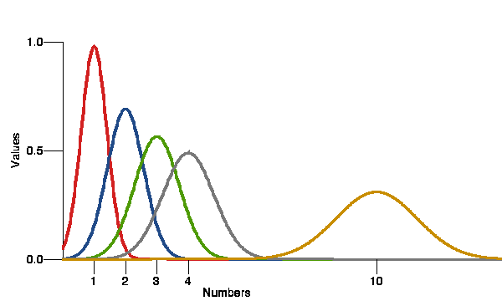
The numerals of a number system exemplify modularity with a module of the number one and all the other numerals being multiples of that number. Place value number systems, like our base 10 system, also give rise to a hierarchy of larger sized units: decades, hundreds etc.

Figure 1: Cuisenaire Counting Rods
Cuisenaire counting rods are a direct physical representation of this relationship, with one size and colour of rod for each of 1 to 10 numbers with length and colour encoding number.

Figure 2: The Evolving House. Vol. III. Rational Design (from Bemis A. F. 1937, p71)
The much-referenced images above, by Albert F. Bemis, merely show that with a small enough module it is possible to describe all the structural elements of a house. Prefabrication and standardisation efforts assume that it is desirable to reduce the variety and number of necessary components in a building programme. Repetition of recognisable physical units of similar size or proportion might also be considered aesthetically desirable. The use of multiples of module sizes can reduce component variety and, by using a modular grid, control their location both horizontally and vertically. However, the horizontal and vertical modules do not need to be the same and as shown later often reflect quite different functional requirements.

Figure 3: Modular Fixing and Location Grids
House Design Program
The Scottish Special Housing Association (SSHA) and the Edinburgh University Architectural Research Unit (ARU) developed a Computer Aided Design program, called House Design. (Bijl et al., 1971) Whilst working at Edinburgh University and SSHA, I was mainly responsible for the practical implementation of this program particularly simplifying the interactive positioning of components
House Design allowed experienced designers to interactively design house types within Circular 36/69 restraints, which had already been incorporated, with some minor variations, into the Scottish Building Regulations.
All location, component and assembly drawings and bills of quantities were then automatically produced without further interaction, by reference to a complete set of standard component and assembly details. That is all possible component and assembly details had been identified, detailed and quantified in advance of their being required.
External walls, windows and external doors were located by placing pairs of 300mm square symbols constrained to be within a 300 mm grid. Structural partitions, non-loadbearing partitions and internal doors were located by placing pairs of 100mm square symbols constrained to be within a 100mm sub-grid. External walls, windows and external doors were therefore notionally 300mm wide whilst structural partitions, non-loadbearing partitions and internal doors were notionally 100mm wide.

Figure 4: House Design: Grid Based Component Location
Extra information such as window height or door swing direction was supplied by pulldown menus or extra pointing. At the time this was described as being a 2½D model; most information being derived from the 2D plan with some default height information and a little extra input to supply information about the 3rd dimension.

Figure 5: House Design: Vertical Dimensions
Of particular importance was the adoption of a standard 2600mm floor to floor height. This allowed stair symbols and floor openings to be accurately known. Thus far, this all conformed to Design Bulletin 16: Dimensional Coordination in Housing (MoHLG, 1969). Problems arose though when actual component widths differed from their 300 or 100mm notional widths.

Figure 6: House Design: Symmetrically Located Components
Without finishes, external walls were actually 240mm wide rather than 300mm, structural partitions 74mm wide rather than 100mm and non-loadbearing partitions 50mm wide rather than 100mm. Design Bulletin 16 recommended (probably required) that internal components were located with their finished faces on a 100mm grid line. Somewhat surprisingly it was thought that this would aid the location of components on site, perhaps assuming that they would all be pre-finished and in modular lengths.
Locating components symmetrically within their grid space with 30, 13 and 25mm offsets as illustrated above, meant that location plans could be automatically dimensioned, with dimensions to the structural face of the components, that is before plasterboard etc. was fixed and exactly as site operatives found them. This meant that as shown below grids could be ignored on site and not shown on location drawings; their work having been done in organising the system, they were no longer needed and could be discarded.
The use of 300 and 100mm grids did however usefully reduce the number of component sizes especially for windows, external doors (300mm increments) and internal doors (100mm increments). This was at the expense of non-modular partition lengths which in any case were less likely to be manufactured off site.
It is probably worth saying that modern production methods mean that components, like doors, can be produced to almost any dimension. Apart from the need to have perceivable visual order, this transfers site assembly problems to identifying slightly varying components and the difficult logistics associated with ensuring that individual components are delivered as and when required.

Figure 7: House Design: Accurately Dimensioned Location Drawing
Detail Complexity
The requirement to locate components with their finished faces on grid greatly increases the number of assembly details that are required. The enumerative analysis that follows was used to justify locating components symmetrically within their grid zones rather than face on grid.
The diagram below shows all the possible ways internal components can meet when they are located symmetrically within a grid. The numbers in brackets indicate the number of ways that components in that configuration can meet if they are located face on grid.

Figure 8: Possible Symmetrical Partition Locations
The following diagram, not part of the original analysis, shows the 16 ways components in the circled arrangement above, can meet when they are located with their faces on grid.

Figure 9: Possible Face On Grid Partition Locations for Circled Configuration
In summary, locating internal components symmetrically within their grid space reduces the number of assembly details required by a factor of almost 8 and thereby avoids the need for lots of otherwise very similar and potentially confusing details.
Combinations of Numbers in Building
As another means of reducing the number of required components, Combinations of Numbers in Building (Dunstone, P. H. 1965) demonstrates the way small numbers of modular components can be used in combination to satisfy the requirement of filling a continuous series of modular sizes. For instance, in the example below what modular spaces can be filled with two components that are 3 and 5 modules long? With these lengths it is not possible to fill spaces of 4 or 7 modules, but it is possible to fill all modular spaces of 8 modules or more. Making 8 what Dunstone calls the Critical Number (CN) for these sizes.

Figure 10: Combinations of Numbers in Building (after Dunstone, P. H. 1965, p.20)
In the days before computers or pocket calculators, Dunstone produced a number of graphical tools to aid in selecting appropriate component sizes to give particular Critical Numbers. However, the Critical Number for two integer modular sizes a and b can easily be calculated as follows, CN = (a – 1) x (b – 1). In the example given above CN = (3 – 1) x (5 – 1) = 8. With 3 or more sizes the calculations can just be done in pairs and the lowest CN used.
Dunstone gives a number of heuristics for choosing component sizes but surprisingly given what follows correctly warns that if two component sizes of a trio, combine to make a third in Fibonacci series fashion (e.g. 3, 5 and 8) then the CN of the trio is not reduced by the third member but the number of ways individual sizes can be made up is increased.
In my early professional career, I used this procedure to design a prefabricated foundation system for the MoHLG Research and Development Group’s Finchampstead Project. A small number of modular beam lengths were selected that could be arranged in different ways so that all modular block lengths and depths could be accommodated, and foundation pads always placed so as to avoid the position of service entry plugs and soil stacks, which were the only things allowed to pierce the ground floor slab.

Figure 11: Finchampstead Project: Foundation Design
Proportion
Proportion can have practical as well as aesthetic uses. In particular, a number of rectangles with specific aspect ratios can be recursively divided into rectangles with the same aspect ratio. This implies that these rectangles can be inflated as well as divided, that is become part of a larger rectangle with the same aspect ratio. The diagram below illustrates the three rectangles that can initially be divided into two such rectangles. In each series, equal aspect ratios are indicated by diagonal lines and squares by inscribed circles.

Figure 12: Recursively Dividing Rectangles in Two
The rectangle with a root 2 aspect ratio, on the left above, allows itself to be split in half across its longer edge to give 2 rectangles with the same aspect ratio, a process that can be repeated ad infinitum. This is the ratio underlying the A series of paper sizes, A1 is half A0 etc. and all sizes usefully have the same aspect ratio. Something that seems satisfying in both aesthetic terms and the parsimonious use of materials.
The double square 2:1 ratio allows each square to be divided into two rectangles with the same 2:1 aspect ratio, again a process that can be repeated indefinitely. This is the ratio that prosaically underlies standard brick sizes, with coordinating dimensions, including one 10mm mortar joint in each direction, of 225 x 112.5 x 75mm (length x width x height).
The division of the Golden Section rectangle is a little more difficult to describe. This rectangle can be split into a square and a smaller rectangle that has the same aspect ratio, a process that can then continue to be applied repeatedly to the smaller rectangle.
The Golden Section
The value of the Golden Section derives directly from the following relationship, that the ratio of L to S is the same as the ratio of (S + L) to L.

Figure 13: Golden Section Derivation
Although formally the Golden Section Ø is an irrational number and therefore cannot be represented as the ratio of two integers, in fact with any Fibonacci type sequence, where n = (n – 1) + (n – 2), as n increases the ratio n / (n – 1) progressively approaches Ø.

Figure 14: Fibonacci Approximation to Golden Ratio (1)

Figure 15: Fibonacci Approximation to Golden Ratio (2)
(8 / 5) is a fair approximation of Ø but (13 / 8), (21 / 13), (55 / 34) and (89 / 55) etc. are progressively better approximations. Moreover, rectangles drawn with these ratios cannot be visually discriminated from ones drawn more accurately and there would seem to be no point in trying to be more accurate than these integer approximations. The rectangles below were drawn with the same shorter edge and the longer edge scaled to give the stated long to short ratio.

Figure 16: Discriminating the Golden Rectangle
When trying to fit a Golden Rectangle to a classical building like the Parthenon, it always seems difficult to decide what should be included. I think that all that can reasonably be concluded is that the Parthenon has a pleasing proportion that is similar to that of the Golden Rectangle.

Figure 17: The Parthenon and the Golden Rectangle
Tiling the Plane with Aperiodic Tiles
As shown in Shadows of Reality : The Fourth Dimension in Relativity , Cubism , and Modern Thought (Robbin, 2002), the Golden Section (and other irrational numbers like root 2 and the Plastic Number) can play a part in proving that aperiodic tiles tile the plane, see Aperiodic Tiling. These irrational ratios can be used to generate the long and short ‘musical sequences’ that describe large sets of aperiodic tiling.

Figure 18: Musical Sequence from the Golden Section (after Robbin 2002, p.65)
In musical sequences a long interval can follow another long interval, but a short interval must follow two long intervals, and a short interval must be followed by a long one.

Figure 19: Short and Long Relationship
In inflation, or composition, the new short interval is equal to the old long interval and the new long interval is equal to the old short interval plus the old long interval. The substitutions S’ = L and L’ = L + S, mandate the Golden Section L / S = (L + S) / L = Ø.

Figure 20: Inflation of Musical Sequences (after Grünbaum and Sheppard, p.574)
As described in Tilings and Patterns (Grünbaum and Sheppard, 1986), the fact that such inflation (composition) can continue for ever, proves the ability of aperiodic tiling to tile the plane.

Figure 21: Composition of Penrose P2 Tiling (after Grünbaum and Sheppard, 1986, p.573)
In partial explanation as shown below, the Golden Section and Penrose P2 Tiling both have an underlying relationship to the pentagon.

Figure 22: Relation of Pentagon to Ø and Penrose P2 Tiles
V+A Spiral Project and Aperiodic Tiling
Aperiodic tiles were used by Daniel Libeskind and Cecil Balmond in their Victoria and Albert Museum ‘Spiral’ proposal. Ammann A2 tiling was used in a hierarchical fractal manner at different scales for physical surface treatments, tiles and panels. Ammann bars, enforcing aperiodicity, also provided a linear support structure.

Figure 23: Ammann A2 Tiling (after Grünbaum and Sheppard 1986, p.550)

Figure 24: V+A Spiral Project (from Cecil Balmond Studio and Daniel Libeskind Studio)
The use of aperiodic tiles in this project is well documented in Informal (Balmond and Smith, 2007) including this quote from Cecil Balmond (as formatted by him).

Balmond and Smith 2007, p.245.
The Modulor
Richard Padovan in Proportion Science, Philosophy, Architecture (Padovan, 2001) describes the precursors and early development of Le Corbusier’s Modulor. In its later versions the Modulor attempted to do two things, to reconcile the supposedly more anthropometric imperial units with the supposedly more mechanical metric units, and to link human dimensions to the Golden Section, in red and blue doubled scales.

Figure 25: Le Corbusier, The Modulor: 1951, cover
Basically, the Modulor is a vertical scale, relating the height of a rather tall man to the Golden Section, and therefore does not relate particularly to modular planning in the horizontal plane.

Figure 26: Le Corbusier, The Modulor: 1951, p.67
Interestingly Le Corbusier himself carried around a customised tape measure marked with imperial and metric scales on one side and the divisions of the Modulor marked on the other. This looks like an attempt to use the Modulor to find order in the existing world as well as impose order on a future world.

Figure 27: Modulor Tape Measure: Modern Facsimile
BRS Modular Number Pattern
Ezra Ehrenkrantz in The Modular Number Pattern, Flexibility Through Standardisation (Ehrenkrantz, 1956) was concerned about dimensional coordination in the British building industry as a whole. He was aware of Corbusier’s Modulor and its relation to the Golden Section and the Fibonacci Series. Produced before the advent of the personal computer or electronic calculators, he presented his preferred numbers on a set of three separated transparent sheets.

Figure 28: BRS Modular Number Pattern 1 (from Ehrenkrantz, E. 1956, insert)

Figure 29: BRS Modular Number Pattern 2 (after Ehrenkrantz, E. 1956, insert sheets)
The top sheet has the Fibonacci series down the left-hand edge and a doubling series across the top (both in red) with their products in the remaining squares (ignoring anything above 1000). The second sheet has the values on the first sheet multiplied by 3 and the third sheet multiplied again by 3. Whilst the Fibonacci and doubling series might provide useful combinations, it is not clear why the multiplications by three are useful but still only 82 black and 23 grey sizes are suggested.
Based on his experience of the Hertfordshire schools building programme whilst in England and working with the Building Research Station, Ehrenkrantz went on to develop the much lauded Southern California Schools Development program. (Ehrenkrantz, Ezra, 1989) Using a 60” (5’) module all components except the building envelope, but including the structure, mechanical services, lighting and interior partitions were realised as a performance specified, modularly coordinated kit of parts, where parts could be easily assembled, disassembled or reconfigured. The 60” (5’) module giving rise to organised spaces with 10’, 20’ and 30’ dimensions.

Figure 30: SCSD Components (from Ehrenkrantz, Ezra, 1989, p.141)
New Proportional Systems
In a recent Guardian article The golden ratio has spawned a beautiful new curve: the Harris curve (https://tinyurl.com/yxf98lez), Alex Bellos wrote about the American mathematician, Edmund Harris, who has identified a series of proportional systems where rectangles can be split into squares and same aspect ratio rectangles. These include the root 2, Ø and double square rectangles described previously, where the given rectangle is initially divided into two parts. But Harris shows that there is also a further family of proportional systems based on rectangles where the original rectangle is initially split into three parts, that again are either squares or rectangles with the same aspect ratio.
The Golden Rectangle and Double Square examples greyed out below can be thought of as second-generation divisions of their two division parents. The root 2 three-part division, however, is different from the previously described root 2 version in that the rectangle is divided into two different sized squares and a rectangle with the same aspect ratio rather than two rectangles with the same aspect ratio.
The two-division ratios given previously and the ratios below are all solutions to simple equations, sometimes known as algebraic numbers. These equations are given above the top-left corner of each rectangle. For example, the equation for the golden rectangle is x2 = x + 1 and for the Plastic Number x3 = x +1 etc.

Figure 31: Other Proportional Systems
The Plastic Number
We are overwhelmed by nature and we are looking for artificial principles to dissolve this contrast, to again get a grip on space, to again understand and control it. Architecture in this sense becomes a necessary instrument for our intellect as well as an expression of a regained authority, of an understood space.
Van der Laan, 1941
quoted in Caroline Voet, 2016, p.4
The architect and Benedictine monk, Dom Hans van der Laan (1904 – 1991) discovered, or rediscovered, the Plastic Number in 1928 although until 1955 he called it the ‘ground ratio’. Like the Golden Section, the Plastic Number has a related Fibonacci like sequence where n = (n – 2) + (n – 3). This is now called the Padovan sequence (OEIS A90031), named for van der Laan’s biographer, Richard Padovan.

Figure 32: Padovan Series Approximation to the Plastic Number 1

Figure 33: Padovan Series Approximation to the Plastic Number 2
With the Padovan sequence, the (4 / 3) ratio is extremely close to the Plastic Number (being a little more than half a percent off its true value). Consequently, the convergence of the succeeding ratios is not so pronounced as with the Fibonacci series and the Golden Ratio. (4 / 3) is a better approximation to the Plastic Number than either (9 / 7) or (21 / 16) but is not as good as (49 / 37).
The closeness of the (4 / 3) ratio to the true irrational value has led people to describe the Plastic Number theory as an additive system rather than a proportional one or at least an additive system that facilitates pleasant proportions.
Van der Laan himself believed in the philosophical notion of there being a perceptible order in space, that could be revealed in architecture through a commensurable proportional system. He assumed that the minimum ratio between two sizes that could be differentiated was 4:3. By differentiating he meant recognising a difference that can be counted or named. He does not mention Weber’s Law or the Distance Effect but in accounting for the 4:3 preference does refer to their just ‘discernible difference’.

Figure 34: Differentiating Ratios
Van der Laan thought that the Plastic Number was superior to the Golden Section because it produced a continuous series of same proportion divisions (on the right below), whilst the Golden Section when applied repetitively leads to two equal length divisions (on the left below).
He also, according to Padovan erroneously, thought that the Plastic Number was inherently more 3-dimensional than the Golden Section because it was the solution to the equation x3 = x + 1 rather than x2 = x + 1 for the Golden Section.

Figure 35: Golden Section and Plastic Number Ratios
The application of van der Laan’s design philosophy produced a fairly austere, spiritual, although according to him not minimalist, architecture.

Figure 36: St. Benedictusberg Abbey, Vaals, (photo by Coen van der Heiden 2008).
Despite the austere nature of his architecture, van der Laan displayed a playful nature when promoting his theories. For instance, leaving ordered piles of pebbles for his students to find and designing Cuisenaire like sets of proportional wooden bricks.
In an experiment that van der Laan conducted with his students, as shown on the left below, he carefully selected 36 pebbles each of which was 1/25th less in diameter than the previous one, considering this a difference that could be perceived without measurement. He then asked his students to sort the mixed pebbles into sets that appeared to be of the same size, a process shown in the middle column below.

Figuire 37: Hans van der Laan: Number and Ratio (from C. Voet 2016, p.5)
Van der Laan claimed that all his students selected 7 groups of ‘equal’ sized pebbles and that the ratio between the group sizes was 4:3 as shown in the right-hand column above. In Between Looking and Making: Unravelling Dom Hans van der Laan’s Plastic Number,Caroline Voet describes repeating this with her students and not getting quite such clear results. (Voet, 2016)
Van der Laan was particularly interested in the number 7 and the ratio 1:7 which he thought was the maximum difference between two sizes that could still be related, what he called their ‘nearness’.

Figure 38: Nearness and the Ratio 1:7
Using the ratios 3:4 and 1:7 van der Laan produced a series of 8 ‘authentic’ sizes, where each size starting at 4:3 closely approximates to a power of Ψ, the Plastic Number, shown in red below. Van der Laan also introduced a derived set of sizes where each authentic size is coupled with a derived size that is 6/7th of its size.

Figure 39: Plastic Number: Van der Laan’s Authentic and Derived Sizes
In van der Laan’s toy like, Form Banks or Morphotheeks, he uses the authentic range of sizes to create arrays of wooden shapes and volumes, which he classifies as blocks (brown below), bars (yellow), slabs (blue) and blanks (white). Each type also has a representative form, shown in a lighter colour. This resulted in 36 preferred shapes and 122 preferred volumes which designers could play with and come to understand their relationships.

Figure 40: Van der Laan Form Banks

Figure 41: Form Bank (photo Jeroen Verrecht)
Being Commensurate
As with the House Design example above, when communicating sizes on drawings or in instructions it is desirable to use values that are easily understood, that is whole numbers or if necessary, simple fractions like 1/2. The adoption of millimetres as the UK official unit of measure for the building industry greatly facilitates this, the unit being small enough to almost entirely remove the need for fractions.
Padovan’s analysis of the Parthenon below also illustrates the need for dimensions to be commensurate. (Padovan, 2001) He suggests a column spacing of 5 units, a stylobate that is 3 units wide wrapped round a core of 15 x 6 column spacings. Assuming that column edges are aligned with the outer edge of the stylobate and that the corner column spacings are reduced, this gives rise to overall dimensions of 81 x 36 units. A core ratio of 15:6 (5:2) becomes an overall ratio of 81:36 (9:4) but all the important dimensions are small whole numbers.

Figure 42: Parthenon: Whole Number Interpretation (after Pardovan, 2001, p.95)
Another historical example is Palladio’s use of whole numbers of Vicentine feet and occasional simple fractions in his drawings of the Villa Foscari and other villas in his Four Books of Architecture. (Palladio, trans Tavenor and Schofield, 1997)

Figure 43: VillaFoscari (from Palladio, trans Tavenor and Schofield, 1997, p.128)
Conclusions
Repetition can be desirable for both aesthetic and practical reasons. Modularity facilitates repetition of object sizes whilst proportion facilitates repetition of the aspect ratio of shapes in a potentially fractal manner but essentially without size repetition.
Number systems are a natural model for modular sizes, where the module is the number one and the natural numers are its multiples. If the number system is a place value system, see Place Value, then the individual places can provide a hierarchy of larger modules sizes.
Planning grids encourage modularity by regulating the placing and size of building elements, but horizontal and vertical modules do not need to be the same. The way elements are located within their grid space can facilitate appropriate dimensioning and remove the need for grids to be shown on locations drawing. Placing components symmetrically within their grid space also significantly reduces the number of assembly details that are required.
Component variety can also be reduced by carefully choosing modular sizes that can combine together. However, choosing sizes that are related in a Fibonacci like manner does not increase the possible range of sizes but does increase the number of ways that they can be combined.
Whilst proportional systems are all defined by irrational numbers, in practice it is impossible to tell if rational integer approximations have been used in their presentation rather than an approximation to several or many decimal places.
Proportional systems have practical as well as aesthetic uses. For instance, the root 2 rectangle giving rise to A paper sizes and the Golden Section (Ø) being part of the proof that aperiodic tiles tile the plane. Ø and its underlying Fibonacci series also form the basis of Corbusier’s Modular and Ehrenkrantz’s BRS Modular Number Pattern, neither of which seem to have had any lasting effect or legacy.
The fact that the ratio 4:3 is extremely close to the Plastic Number (Ψ) means that the proportional system proposed by Dom Hans van der Laan can usefully bridge the gap between modular and proportional systems.
As shown in the Round and Sharp Numbers post some numbers are round and a slightly different set, relating to the base 10 of our number system, are favourites. These are the numbers that we would naturally prefer to use or find when measuring. Like the House Design example this relates to dimensions needing to be commensurate that is wherever possible whole numbers or simple fractions.

Figure 44: Component Sizes, Favourite Numbers and Greedy Algorithm
Bibliography
Bijl, A. et al. (1971) ARU research project A25/SSHA-DOE: house design ; application of computer graphics to architectural practice, ARU CAAD Studies. Edinburgh Unniversity, Architecture Research Unit, 1971.
Ehrenkrantz, Ezra, D. (1989) Architectural Systems: A Needs, Resources and Design Approach. McGraw-Hill.
Ehrenkrantz, E. (1956) The Modular Number Pattern, Flexibility Through Standardisation. HMSO.
Grünbaum, B. and Sheppard, G. C. (1986) Tilings and Patterns. W. H. Freeman and Company.
MoHLG (1969) Design Bulletin 16: Dimensional Coordination in Housing.
Padovan, R. (2001) Proportion, Science, Philosophy, Architecture.
Palladio, A., trans Tavenor, R. and Schofield, R. (1997) The Four Books of Architecture. The MIT Press.
Robbin, T. (2002) ‘Shadows of Reality : The Fourth Dimension in Relativity , Cubism , and Modern Thought’, Dimension Contemporary German Arts And Letters, pp. 74–76.
Voet, C. (2016) ‘Between Looking and Making: Unravelling Dom Hans van der Laan’s Plastic Number’, Architectural Histories. Ubiquity Press, Ltd., 4(1), pp. 1–24. doi: 10.5334/ah.119.